
GIZMO
… get off the grid ...
Welcome!
GIZMO is a flexible, massively-parallel, multi-physics simulation code. The code lets you solve the fluid equations using a variety of different methods -- whatever is best for the problem at hand. It introduces new Lagrangian Godunov-type methods that allow you to solve the fluid equations with a moving particle distribution that is automatically adaptive in resolution and avoids the advection errors, angular momentum conservation errors, and excessive diffusion problems that limit the applicability of “adaptive mesh” (AMR) codes, while simultaneously avoiding the low-order errors inherent to simpler methods like smoothed-particle hydrodynamics (SPH). Meanwhile, self-gravity is solved fast, with fully-adaptive gravitational softenings. And the code is massively parallel — it has been run on everything from a Mac laptop to >1 million CPUs on national supercomputers.
The code is originally descended from GADGET, and has retained many naming/use conventions as well as input/output cross-compatibility — if you have code or experience from GADGET, it should immediately be compatible with GIZMO.
Some of the physics modules in GIZMO include:
- Hydrodynamics: with arbitrarily chosen solvers (new Lagrangian methods, or SPH, or fixed-grid Eulerian methods)
- Magnetic fields: ideal or non-ideal MHD, including Ohmic resistivity, ambipolar diffusion, and the Hall effect
- Cosmological integrations: large volume and cosmological “zoom in” simulations, with on-the-fly group finding
- Radiative heating/cooling & chemistry: including species-dependent cooling and pre-tabulated rates from 10-1e10 K, optically thin or thick cooling, consistent (equilibrium or non-equilibrium) ion+atomic+molecular chemistry, and hooks to external chemistry and cooling packages
- Galaxy/Star/Black hole formation and feedback: explicit modules for star and black-hole formation and feedback in galaxy-scale and cosmological simulations including detailed explicit models for jets, winds, supernovae, radiation, and common sub-grid models used in larger-scale/lower-resolution simulations
- Individual Star/Planet sink-particle formation: with explicit proto-stellar and main-sequence evolution and feedback channels (jets, winds, supernovae), designed for individual star and planet formation simulations
- Non-standard cosmology (e.g. arbitrarily time-dependent dark energy, Hubble expansion, gravitational constants), and modules for self-interacting, dissipative, exothermic, primordial black-hole and scalar-field/fuzzy dark matter;
- Self-gravity with adaptive gravitational resolution: fully-Lagrangian softening for gravitational forces, with optional sink particle formation and growth, and ability to trivially insert arbitrary external gravitational fields
- Anisotropic conduction & viscosity: fully-anisotropic kinetic MHD (e.g. Spitzer-Braginskii conduction/viscosity), or Navier-Stokes conduction/viscosity, and other non-ideal plasma physics effects
- Subgrid-scale turbulent “eddy diffusion” models, passive-scalar diffusion, and the ability to run arbitrary shearing-box or driven turbulent boxes (large-eddy simulations) with any specified driving spectrum
- Dusty fluids: explicit evolution of aerodynamic particles in the Epstein or Stokes limits, with particle-particle collisions, back-reaction of dust on gas, Lorentz forces on charged particles, and more
- Degenerate/stellar equations-of-state: appropriate Helmholtz equations of state and simple nuclear reaction networks
- Elastic/plastic/solid-body dynamics: arbitrary equations-of-state with pre-programmed modules for common substances (e.g. granite, basalt, ice, water, iron, olivine/dunite), including elastic stresses, plastic behavior, and fracture models
- Radiation-hydrodynamics: full and flexible, with a variety of modular solvers and the ability to trivially add or remove frequencies to the transported set (pick and choose which wavebands you want to evolve)
- Arbitrary refinement: with new splitting/merging options, you can “hyper refine” in an arbitrarily desired manner dynamically throughout the simulation
- Cosmic Ray transport and magneto-hydrodynamics. Modular choices of solvers for cosmic ray transport, and full coupling to gas including cooling and adiabatic, diffusion, Alfven-wave coupling, streaming, injection, and more.
- Particle-in-Cell simulations: using the hybrid MHD-PIC method where species such as cosmic rays with large gyro-radii are integrated explicitly, while the background tightly-coupled electrons are integrated in the fluid limit
- Other in-development features include detailed nuclear networks, relativistic hydrodynamics, and more
Important Links:
The publicly-available version of the code (hosted on a Bitbucket repository). It has full functionality for the “core” physics, including almost all physics listed above. This is intended for a wide range of science applications, as well as learning, testing, and code methods studies. A few modules are not yet in the public code, because they are in active development and not yet de-bugged or tested at the level required for use “out of the box” (but will be made public as soon as this stage is reached). In a few cases it is because they involve proprietary code developed by others with their own collaboration policies, which must be respected (see User Guide for details).
Everything you need to know to run and/or analyze simulations with GIZMO. Includes a suite of examples and test problems as well. If you have questions/bug reports/etc that go beyond the user guide, please join the GIZMO Google Group.
The GIZMO code/methods paper explains the hydrodynamic methods in detail and explores them in a large suite of test problems. Because there are many different physics modules in GIZMO, there are different methods papers for different code modules (for example, the GIZMO-MHD code/methods paper, which explains the implementation of ideal magneto-hydrodynamics). You should always read the appropriate methods paper[s] before using any given module, and cite them in papers using them! Links to the appropriate papers for each part of the code are in the User Guide. A broader overview of different numerical methods (suitable for an introduction before diving into the more detailed code papers) is available from one of my talks here.
If you wish to contribute to active development or new physics in GIZMO, you can branch off the public code, and eventually push to the development (not public) version of the code which is hosted on a separate Bitbucket repository here. For permissions you will need to contact me directly; if you do, please include an explanation of your plans and why you want to be involved in development.
Publications:
Explore recent publications using and citing our GIZMO (and earlier P-SPH) methods papers (on NASA ADS)
Examples:
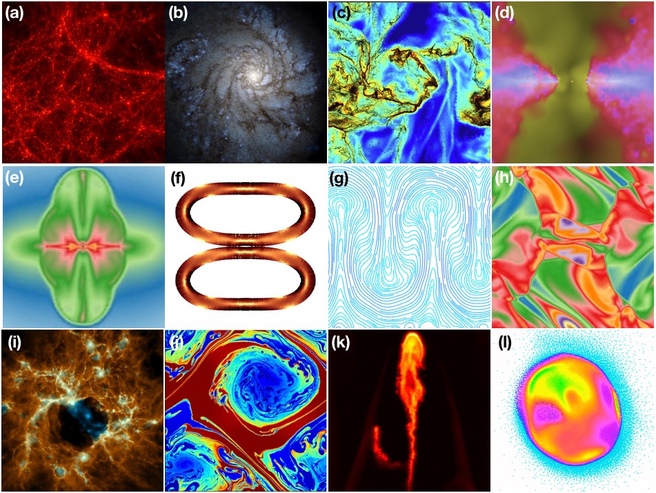
GIZMO and its methods have been used in a large number of simulations and well over a hundred different papers (for a partial list of works which reference the original methods paper, click here). Some examples are shown above, including: (a) Cosmology: Large-volume dark matter+baryonic cosmological simulation (Davé et al. 2016).
(b) Galaxy formation: with cooling, star formation, and stellar feedback (Wetzel et al. 2016). (c) Dust (aero)-dynamics: grains moving with Epstein drag and
Lorentz forces in a super-sonically turbulent cloud (Lee et al. 2017). (d) Black holes: AGN accretion according to resolved gravitational capture, with feedback
driving outflows from the inner disk (Hopkins et al. 2016). (e) Proto-stellar disks: magnetic jet formation in a symmetric disk around a sink particle, in non-ideal MHD (Raives 2016). (f) Elastic/solid-body dynamics: collision and compression of two rubber rings with elastic stresses and von Mises stress yields. (g)
Plasma physics: the magneto-thermal instability in stratified plasma in the kinetic MHD limit (Hopkins 2017). (h) Magneto-hydrodynamics: the Orszag-Tang
vortex as a test of strongly-magnetized turbulence (Hopkins & Raives 2016). (i) Star formation: star cluster formation (with individual stars) including stellar
evolution, mass loss, radiation, and collisionless dynamics (Grudic et al. 2016). (j) Fluid dynamics: the non-linear Kelvin-Helmholtz instability (Hopkins
2015). (k) Multi-phase fluids in the ISM/CGM/IGM: ablation of a cometary cloud in a hot blastwave with anisotropic conduction and viscosity (Su et al.
2017). (l) Impact and multi-material simulations: giant impact (lunar formation) simulation, after impact, showing mixing of different materials using a
Tillotson equation-of-state (Deng et al. 2017).
Some advantages of the new methods in GIZMO:
Angular Momentum Conservation:
Can we follow a gaseous disk?
Let’s consider what should be a straightforward test problem, of enormous astro-physical importance. A cold, inviscid, ideal-gas disk (pressure forces less important than the global gravitational forces on the gas) orbiting in a Keplerian (point-mass) potential on circular orbits, with no gas self-gravity. The gas should be stable and simply orbit forever. But what actually happens when we numerically evolve this?
“Standard” (non-moving) fixed-mesh or adaptive mesh codes:
Left: This movie shows the test problem, in a non-moving “grid” code (here, the code ATHENA). The movie shows the gas density, from 0 (black) to 2 (red). The initial condition has density =1 (green) inside a ring (the hole and outer cutoff are just for numerical convenience). We’ve set things up so it’s the “best case” for this sort of code: the resolution is high (256^2), we use a high-order method, and disk is only 2-dimensional and is perfectly aligned in the x-y Cartesian plane (so we don’t worry about vertical motion). The movie runs from t=0 to t=100 in code units, or about 10 orbits of the middle of the ring.
Almost immediately (within ~1 orbit) the disk starts to break up catastrophically. We can change the details by changing things like the order of the method, but it only makes things worse (the disk can look smoother, but all the mass diffuses out in the same timescale!). The problem is that mass must constantly be advected across the grid cells (at irregular angles, too). AMR-type codes do not conserve angular momentum, and have significant advection errors; so the disk breaks up and can’t be reliably evolved for much more than an orbit. Of course, you can help the problem by going to higher resolution, but the test problem here (because its so simple) is already much higher-resolution than most state-of-the art simulations of real problems! And in 3D, you also have a nasty grid-alignment effect: even at extremely high-res (>512^3) in AMR codes, the disk is torqued until the gas aligns with one of the Cartesian axes.
These are serious problems in almost all cosmological, or binary merger, or proto-planetary disk simulations -- anything where the disks should live a large number of orbits. If you’re lucky and can make a problem where you know the problem geometry exactly ahead of time, you can do better (using e.g. a cylindrical mesh) -- but that severely limits the usefulness of these methods.
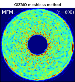
With GIZMO:
The new methods we’ve developed for GIZMO avoid these errors entirely. One of the major motivations for the code was to develop a method which would conserve angular momentum accurately on general problems, and it makes a huge difference!
Right: The same simulation, evolved five times as long (~100 orbits)! The disk evolution is almost perfect: theres some noise, but almost no diffusion of the outer or inner disk, and angular momentum is nearly exactly conserved in both rings and total. Since there’s no grid, there’s also no “grid alignment” in 3D. And the conservation is great even at very low resolution: a 64^2 disk looks almost as good!
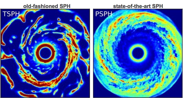
What about SPH?
If you want, you can use GIZMO to run your problem with the smoothed-particle hydrodynamics (SPH) method. In principle, SPH conserves angular momentum. But in practice, to make SPH actually work for real problems, you need to add an “artificial viscosity.” And an artificial viscosity prescription which allows you do deal with shocks correctly almost always leads to too much shear viscosity (which should be zero) in a flow like this. That triggers the “viscous instability” where sticky bits of the disk lead to it breaking up again.
Here, we see that: Left panel uses the old-fashioned “standard” artificial viscosity with a Balsara switch (density shown again, at time t~100). The disk breaks up catastrophically in ~2-3 orbits (but for different reasons than in the grid codes). Right panel uses the “state of the art” in SPH, a higher-order artificial viscosity “switch” from Cullen & Dehnen. Its much better than old-fashioned SPH or AMR codes, but the disk still starts to break up in ~5 orbits or so.
The Kelvin-Helmholtz Instability:
Standard Non-Moving Mesh GIZMO Meshless Method
Here’s a side-by-side comparison of a high-resolution (512^2) simulation of the Kelvin-Helmholtz instability, with the same initial conditions, but using two different numerical methods to solve the equations of motion. Two fluids (one light, one heavy) are in relative shear motion. The gas density is plotted, ranging between 1 and 2 (blue and red). On the left, a non-moving grid (from ATHENA). On the right, GIZMO’s new meshless finite volume method. Both develop the instability (correctly) at the same time, but in the code with a non-moving, Cartesian mesh, the contact discontinuities must be transported at irregular angles across the cells, which leads to a lot of (incorrect) excess diffusion even at this very high resolution, until the rolls simply “diffuse into” each other (in other words, the contact discontinuity cannot be maintained on small scales), and the whole instability blurs into a smooth “boundary layer” between the two fluids. With the new method, these discontinuities can be followed in exquisite detail. In fact, we had to massively down-grade the resolution on the right to make this movie (while, because of all the diffusion, there isn’t any detail lost on the left)! Click here for a higher-resolution version of the movie.
Here is a zoom-in of just part of one of the KH “whorls” -- still downgraded in resolution! Follow this link to get the a PDF with the full-resolution image of the final snapshot time.
What about SPH?
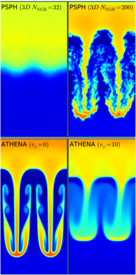
It’s well known that old-fashioned “traditional” SPH has serious problems with the KH instability, and many other subtle fluid instabilities (famously, for example, the magneto-rotational instability). Here the left and right panels show “traditional” (GASOLINE or GADGET-2 type) and “modern” SPH (labeled TSPH and PSPH, respectively). “Modern” SPH refers to SPH using our more accurate “pressure” formulation of the equations of motion (Hopkins), fully conservative corrections for variable smoothing lengths (Springel), a higher-order smoothing kernel (Dehnen & Aly), artificial conductivity terms (Price), higher-order switches for the diffusion/viscosity/conductivity terms (Cullen & Dehnen), and more accurate integral/matrix-based gradient estimators (Garcia-Senz, Rosswog).
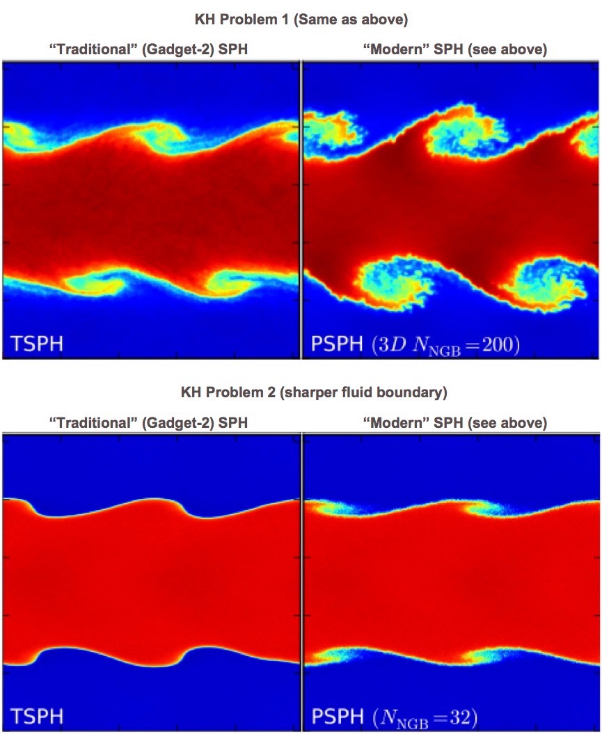
In “traditional” SPH, we see the usual problem. If the seed perturbation is small, the low-order errors of the method suppress its growth (the ‘surface tension’ effect in particular is dramatic) and lead to almost no mode growth. In “modern” SPH, the situation is tremendously improved. However, it still is not perfect: the mode amplitude is not exactly correct, and there is some unphysical “jagged” noise resulting from the artificial conductivity terms. More importantly, even in modern SPH with all the other improvements present, only going to very large SPH neighbor number can “beat down” the zeroth-order errors in quantities like the pressure gradients. Thus, if we re-run with a low initial mode amplitude (say, sub-percent, as opposed to a large ~10% initial perturbation), with the same neighbor number (number of particles the SPH particle must “talk to” each hydro interaction) as our GIZMO methods (32, in this problem), we see dramatic suppression of the KH instability! But going to large neighbor numbers is very expensive. And if we wanted to capture a still-smaller amplitude mode, we’d have to go to higher neighbor number still! And in the GIZMO MHD methods paper, we show these problems are exacerbated for SPH-MHD — accurately capturing phenomena like the MRI (as well as higher-order phenomena in fully-anisotropic kinetic MHD like the MTI or HBI) is straightforward in the new methods in GIZMO, but extremely difficult (if not impossible) in the variants of SPH we have explored.
What about AMR?
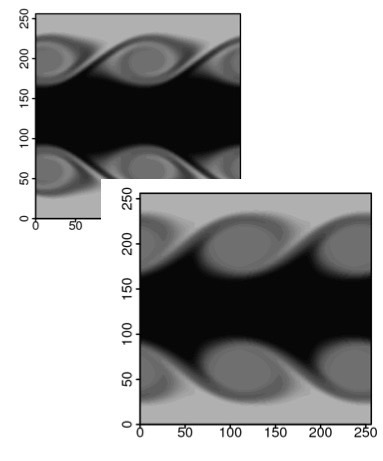
Finally, just in case you’re wondering, going to Adaptive Mesh Refinement (AMR) schemes doesn’t actually help with the problems we described for grid/non-moving mesh codes. The reason is that, unless you just refine everywhere over and over (i.e. just increase the resolution of the simulation -- that’s cheating!), the contact discontinuities will still end up irregularly distributed over and moving over the cartesian mesh edges. It’s not a matter of missing “more cells” in a dense region. This shows that, by showing a grayscale density projection of one of the same tests run in the AMR code RAMSES. The serious diffusion affecting the rolls is obvious -- in fact, its worse here, because at refinement boundaries AMR codes become effectively lower-order accurate.
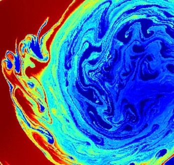
Some Other Examples:
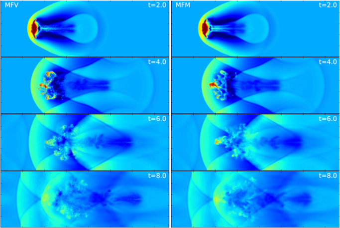
The “blob test” - showing a cold cloud being disrupted by a supersonic wind. The two methods (left and right) are two different GIZMO methods -- both capture the correct physical destruction of the cloud in this test.
Fluid Mixing & Galilean Invariance:
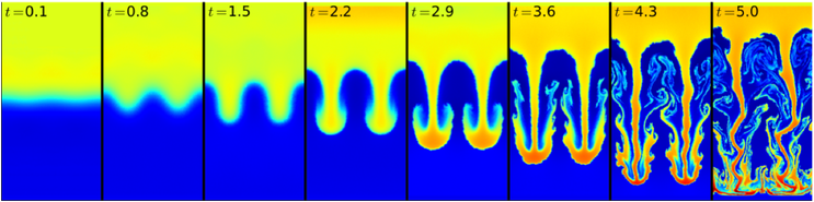 Evolution of the Rayleigh-Taylor instability in our new GIZMO method: balancing a heavy fluid against gravity on top of a light fluid. The instability develops and buoyant plumes rise up, triggering secondary Kelvin-Helmholtz instabilities.
This is what the same instability looks like at time =3.6 in other state-of-the-art methods.
Top Left: “Modern” SPH (as described above), but using the same number of neighbor particles as our GIZMO method. Because of low-order errors in SPH, the method simply cannot capture small-amplitude instabilities (or numerically converge) without dramatically increasing the number of neighbors inside the interaction kernel (greatly increasing the CPU cost).
Top Right: Modern SPH, with a higher-order kernel with many more neighbors. Now the instability is captured, but low-order errors still corrupt the short-wavelength modes (giving them their odd boundaries)
Bottom Left: A static (non-moving) mesh result. Here things look quite nice, even though there is more diffusion in the “rolls” of the secondary Kelvin-Helmholtz instabilities that develop
Bottom Right: The same non-moving mesh, if we simply “boost” the system (set all the fluid in uniform motion). The solution should be identical, but since the fluid is now moving across instead of with the grid, the diffusion is dramatically amplified and the instability is suppressed. We have to go to >10,000 times as many cells to recover the same accuracy! GIZMO, being Lagrangian, has no such velocity-dependent errors.
Implosions & Explosions:
Escaping Carbuncles
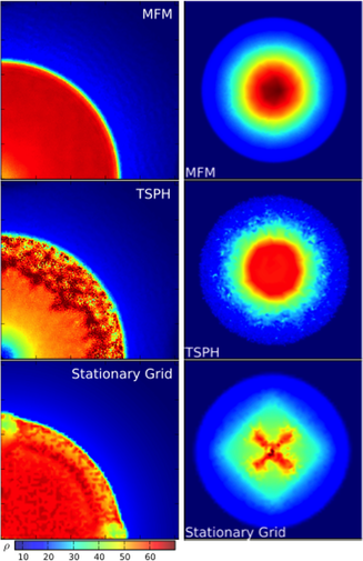
Here are two tests involving strong super-sonic shocks (projection of density). Left is the Noh implosion test (fluid rushing to the origin at infinite Mach number). The box is spherical, but we just show a slice through the x-y plane, and show one quadrant. Right is the Sedov-Taylor explosion (the result of a massive point injection of energy; now the full x-y plane is shown).
Top: MFM is one of our new GIZMO methods. Note that both solutions display excellent symmetry, smooth flows and well-resolved shock fronts.
Middle: SPH. The symmetry is statistically good, but there is far more (unphysical) noise, because of SPH’s low-order errors. Also, some “wall-heating” leads to the cavity in the center of the Noh test.
Bottom: Grid methods. Here there is more noise still than MFM, and more obviously, severe “carbuncle” and “grid alignment” instabilities, where the Cartesian grid imprints special directions and locations along the grid axes instead of the correct spherical structure!
Arbitrary Meshes (Making the mesh move how you want):
GIZMO is truly multi-method in that the "mesh" over which the fluid equations is solved can be specified with arbitrary motion or geometry (or lack thereof). GIZMO can be run as a Lagrangian mesh-free finite-volume code (where the mesh moves with the fluid as described above). But you can also run it as an SPH code (using state-of-the-art SPH methods) — these are some of the examples shown above or in the methods paper. More radically, you can run it as a fixed Cartesian-grid code (or otherwise fixed-grid code), similar to codes like ATHENA or ZEUS (where the cells are fixed cuboids, and do not move, but the fluid moves over them). Even more generally, users can, in fact, specify any background mesh motion they desire — you can easily set up shearing, expanding, collapsing, accelerating, or differentially rotating boxes, for example, to match the bulk motion in your problem. Some examples of these meshes are shown below:
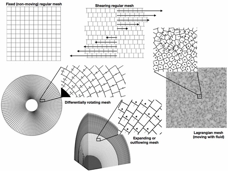
Although the discussion above describe many advantages of "Lagrangian” methods (where the mesh moves with the fluid) for problems with large bulk motion, advection, gravitational collapse, etc, there are certainly many problems where fixed (non-moving) grids can still be advantageous (if the grid is well-ordered or regular). Or where you would like the grid to move with the average flow, but maintain regular structure (such as e.g. a uniformly shearing Cartesian grid). For example, on problems where you wish to follow highly sub-sonic motion accurately, moving meshes generate "grid noise" because the mesh is constantly moving and deforming. This deformation of the system generates pressure fluctuations on a scale of order the integration error, which in turn launch sound waves, that can significantly corrupt the desired behavior. A regular (e.g. Cartesian) non-moving mesh has no "grid noise" however, so avoids these issues. Of course, the method is more diffusive if the grid is not moving, especially if there is substantial advection across the cells, and one has to be careful about imprinting preferred directions on the flow. But in general, in problems where it is very important to maintain a "smooth" background flow (e.g. reduce noise at all costs, even at the cost of significant numerical diffusivity), this can be useful.
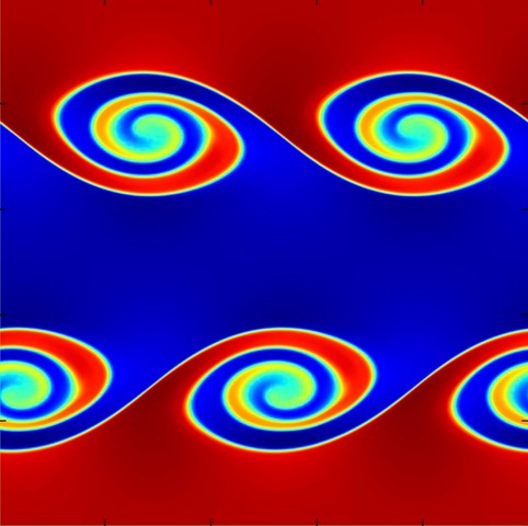
For example, the image at left here shows an example of the non-linear KH instability set up with a smooth boundary, exactly symmetric initial conditions, finite Reynolds number (explicit viscosity), and a single-mode perturbation, following Lecoanet et al. 2016 (MNRAS, 455, 4274). This setup should not, in fact, exhibit the secondary instabilities of the inviscid KH instability shown above, but should maintain “smooth” rolls. As many authors have shown, fully-Lagrangian codes have difficulty avoiding grid noise that seeds secondary instabilities. We show the image of the simulation at just 256^2 resolution in GIZMO, run as a fixed-mesh code, where this is achieved rather easily (results are comparable to ATHENA).
Code Scaling & Performance:
GIZMO uses a hybrid MPI+OpenMP parallelization strategy with a flexible domain decomposition and hierarchical adaptive timesteps, which enable it to scale efficiently on massively-parallel systems with problem sizes up to and beyond many billions of resolution elements. In addition, we have implemented a large number of optimizations for different problems and physics, including e.g. rolling sub-routines and communication together, implementing problem-specific weighting schemes for domain decomposition, solving gravity with a hybrid tree-nested particle mesh approach, and adopting fully adaptive spatial and time resolution. Remarkably, despite the additional computational complexity, the new fluid solvers are actually faster in GIZMO than their SPH counterparts, owing both to the reduced neighbor number needed and to several custom optimizations.
Code scalings are always (highly) problem-and-resolution-dependent, so it is impossible to make completely general statements about how GIZMO scales. However, we can illustrate one example here. This shows the code scalings of GIZMO (in hybrid MPI+OpenMP mode) on full production-quality FIRE-2 cosmological simulations of galaxy formation, including the full physics of self-gravity, hydrodynamics, cooling, star formation, and stellar feedback (from Hopkins et al. 2017, arXiv:1702.06148). This is an extremely inhomogeneous, high-dynamic-range (hence computationally challenging) problem with very dense structures (e.g. star clusters) taking very small timesteps, while other regions (e.g. the inter-galactic medium) take large timesteps — more “uniform” problems (e.g. a pure dark-matter only cosmological simulation or pure-hydrodynamic turbulence simulation) can achieve even better scalings.
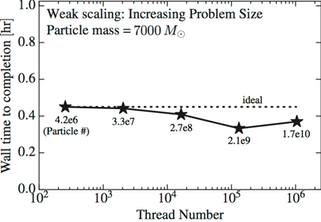
Weak scaling (making the computational problem larger in size, but increasing the processor number proportionally) for a full cosmological box, populated with high resolution particles (fixed particle mass), run for a short fraction of the age of the Universe. We increase the cosmological volume from 2 to 10,000 cubic comoving Mpc. In these units, theoretically “ideal” weak scaling would be flat (dashed line shown). The weak scaling of GIZMO’s gravity+MHD algorithm is near-ideal (actually slightly better at intermediate volume, owing to fixed overheads and statistical homogeneity of the volume at larger sizes) to greater than a million threads (>250,000 CPUs and >16,000 independent nodes).
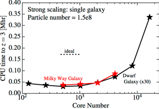
Strong scaling (CPU time on a fixed-size problem, increasing the processor number) for a "zoom-in” simulation of a Milky Way-mass galaxy (1e12 solar-mass halo, 1e11 solar-masses of stars in the galaxy) or a dwarf galaxy (1e10 solar-mass halo, 1e6 solar-masses in stars in the galaxy), each using 1.5e8 (150 million) baryonic particles in the galaxy, run to 25% of the present age of the Universe. In these units, “ideal” scaling is flat (dashed line), i.e. the problem would take same total CPU time (but shorter wall-clock time as it was spread over more processors). Our optimizations allow us to maintain near-ideal strong scaling on this problem up to ~16,000 cores per billion particles (~2000 for the specific resolution shown).
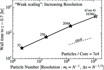
Test increasing the resolution instead of the problem size (specifically, increasing the particle number for the same Milky Way-mass galaxy, while increasing the processor number proportionally). Because the resolution increases, the time-step decreases (smaller structures are resolved), so the ideal weak scaling increases following the dashed line. The achieved scaling is very close to ideal, up to >16,000 cores for ~1 billion particles.
GIZMO: Check It Out!